Whew, that was too much algebra! But we needed to introduce infinite-dimensional vector spaces in order to understand what a Cameron-Martin space is. Like before, you’ll find Alessandra Lunardi (2015) has more mathematical rigor, which we ditched long ago in favor of pedagogical clarity. The gap is significant, though. If you browse Wikipedia, the number of concepts you need to learn to even make sense of a sentence is hard. Hopefully, this will give you enough background on Cameron-Martin to proceed to the Malliavin Derivative.
Gaussian measures
We mentioned last time that we would solve the problem of calculating length and distance of infinite-dimensional vectors (such as functions) by changing the measure from Lebesgue to Gaussian. There’s another reason for that choice, encapsulated in Wikipedia contributors (2024). The Lebesgue measure is the only measure in finite-dimensional spaces that’s:
Locally finite, that is, every set around a point has a finite measure. \(\lambda(N_x) < +\infty\)
Translation invariant, that is, moving a set on a certain direction \(d\) keeps the measure value intact. \(\lambda(\{N_x\}=\lambda(\{N_x "+" d\})\)
Strictly positive, that is, if \(A \neq \emptyset\), then \(\lambda(A)>0\)
For infinite dimensions, there’s no equivalent1. In fact, for most of these spaces the only locally finite, translation invariant measure is the trivial measure \(\mu(A)=0, \forall A\) .
So, we turn to the Gaussian measure, which has exponential tails that can squash function values if they are far away from the center2. But that means we need to address other problems. In particular, the lack of translation invariance.
Translation (in)variance
To better illustrate this issue, let’s assume some kind of Riemann integration like so:
\[
\int_{-\infty}^{+\infty}f(x)dx
\]
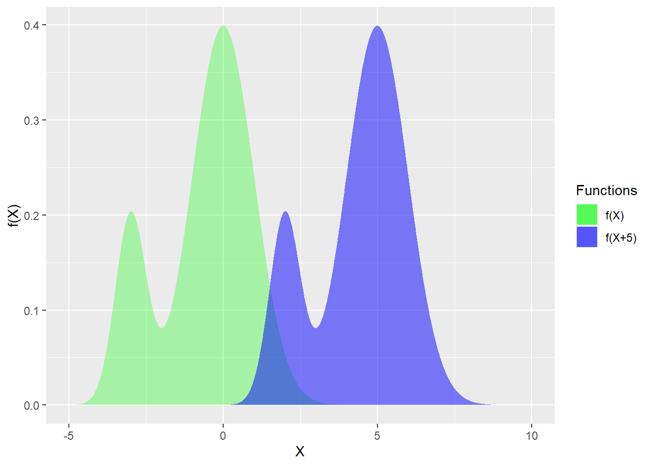
We will now make a change of variable due to a translation \(x \rightarrow x +h\), then the area under the curve will not have changed, it just shifted to the side:
And it finally be confirmed visually. Look at these functions that kind of resemble ghosts. Regardless of the shift, they have the same area under the curve:
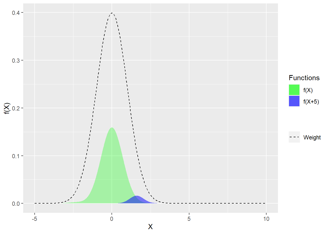
Unfortunately, the Gaussian measure doesn’t allow that. Let’s remember the \(n\)-dimensional or 1-dimensional cases for a standard, centered Gaussian measure.
As you can see, the first function had plenty of area in the middle of the weight, so it retains quite a bit. The shifted function instead has shrunk. Now, even though the area has changed, we could in theory recover the factor by which it has changed. With finite dimensions, this is doable, but it’s challenging in infinite dimensions.
The main idea here is that you are allowed to perform these translations in infinite dimensions and arrive to a calculation that still works. The only requirement is that the translation comes from a “smaller” space, the Cameron-Martin space, and only those translations make sense and are allowed.
The Cameron-Martin space
Although it sounds mysterious, it’s actually kind of straightforward, and you can follow the approach from Wikipedia contributors (2023) and Alessandra Lunardi (2015). Let’s go back to the inner product instead of using the norm, to understand what’s going on, and we will use a finite \(n\)-dimensional space:
So, a Gaussian measure for a translated set is the measure for the original set, multiplied by an extra factor to perform the “change of variable”. That extra factor is called the Radon-Nikodym derivative because it expresses how a measure changes when another changes. In this case, we will denote it as the one that transforms the centered Gaussian measure into the \(h\)-Translated Gaussian measure, symbolized as \(\frac{\partial(T_h)_*(\gamma)}{d\gamma}(x)\)
Now, let’s point out once again that, if there’s a space \(E\) and a measure \(\mu\) that’s locally finite and equivalent to itself after any translation “change of variables”, then either \(E\) is finite-dimensional, as shown above, or \(\mu\) is the trivial measure \(\mu(A) = 0,\, \forall A\). We can also already see from the expression above that if \(h\) is infinite-dimensional then there’s the potential to make this integral tend to infinity. Fortunately for us, we can sidestep this by only expecting equivalence under some translations, namely translations that are elements of a Cameron-Martin space, also called Cameron-Martin directions.
We start from an infinite-dimensional space \(H\), our Cameron-Martin space. We will have \(h \in H\), with a mapping \(i(h):H\rightarrow E\), and \(i(H) \subseteq E\). These \(i(H)\) will be our Cameron-Martin directions. We will impose additional restrictions on \(h\). For starters, and based on the Radon-Nikodym derivative we see above, we need at least\(\|h\|^2_H < \infty\). Then, we need to decide what \(\langle h, x \rangle\) even means and what to do with it. In fact, this isn’t a true inner product because \(h \in H\) and \(x \in E\) (remember, the whole point of \(H\)is to reduce the space!). In short, what’s going on with that fake inner product is that there’s a mapping for every \(h\) to a function in the space of functions \(I(h): H \rightarrow L^2\), and \(I(h)(x)\) is what will count as the “inner product” \(\langle h, x \rangle^\sim\). 3
Example of a Cameron-Martin space
All of the above is pretty arid, so let’s take a look at one example of a infinite-dimensional space and its corresponding Cameron-Martin space. I won’t try to explain how this space was obtained, there’s a lengthy derivation in Alessandra Lunardi (2015) .
Infinite sequences
Recall the space of infinite sequences? It’s an infinite-dimensional space and we denoted it \(\mathbb{R}^{\mathbb{N}}:=\mathbb{R}^{\infty}\), with countable cardinality. Now, let’s consider the space of sequences that vanish at infinity, with the exotic symbol \(\mathbb{R}_c^{\infty}\) and its elements will have the even more exotic symbol \(\xi\in\mathbb{R}_c^{\infty}\) . So, by definition, we know \(\lim_{k\rightarrow \infty}\xi_k = 0\).
Now, we establish a correspondence between these sequences and functions, very straightforward: \(\xi \rightarrow f, \text{with }f(x) = \sum^\infty_{k=1}\xi_k x_k\) , and we will limit this to the sums that are finite, in other words \(f(x)<\infty\) or \(f(x) \in L^2\). Notice that when we measure the first term of this series with a Gaussian measure, we will be simplifying a lot:
Now, you can do this for all \(x_k\) and find the same result. This is no coincidence, and it’s the reason why we used the Gaussian measure for infinite dimensions. In fact, \(\gamma\) for the infinite-dimensional case will have mean \(\mu=0\) and variance/covariance \(B_\gamma(\xi,\xi)=\|\xi\|_{\ell^2}\).
This last statement is also useful because we can use it to arrive from the norm of a function using the Gaussian measure to its value. I won’t prove it now, but \(\|f\|^2_{L^2(X,\gamma)}=\|\xi\|^2_{\ell^2}\). Now, if we take a \(h\in \mathbb{R}^\infty\), we can show (but we won’t) that by having \(h\in H = \ell^2\) instead, this is enough for the functions above to be measured and to always obtain a value. So, the Cameron-Martin space is \(\ell^2\).
Strictly speaking, you can get an analogue, but the space must be non-separable and the measure won’t be sigma-finite. The spaces we deal with will normally be separable. In particular, Hilbert spaces (spaces with inner products that are complete under the metric induced by the inner product) are separable if there’s an orthonormal basis on \(\mathbb{N}\).↩︎
This is called the Paley-Wiener integral. We won’t need to mention or refer to this again because it agrees with the Ito integral when both are defined, similar to the Borel and Lebesgue measures.↩︎