As I mentioned previously, Malliavin Calculus isn’t a topic that can easily relate to everyday things. Most authors I’ve checked don’t detail too much on why an object like it exists, or the Clark-Ocone formula. Instead, they go to the Hormander condition, which is meaningless for our purposes.
If Malliavin Calculus is called the extension of calculus of variations to stochastic processes, then the time has come to discuss stochastic processes and martingales.
Stochastic processes
We can think of stochastic processes as a sequence of random variables that are indexed by time. I’ll start with a very simple case, the one-dimensional random walk (also known as the drunkard’s walk):
This is very simple: at time \(i\), after \(\Delta t\) has passed, the drunkard take a step \(X_i\), which can be either up or down the street with equal probability. The position \(Z\) at \(t\) is simply the result of all the steps the drunkard has taken before. As it stands, each movement “up” can be considered a “success”, so this sum follows a binomial distribution centered at \(0\).
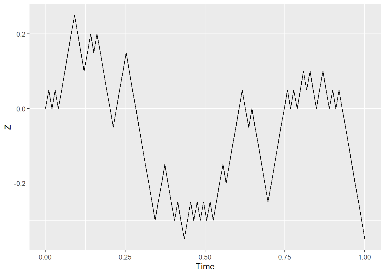
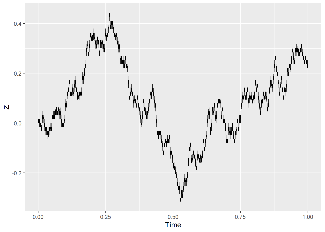
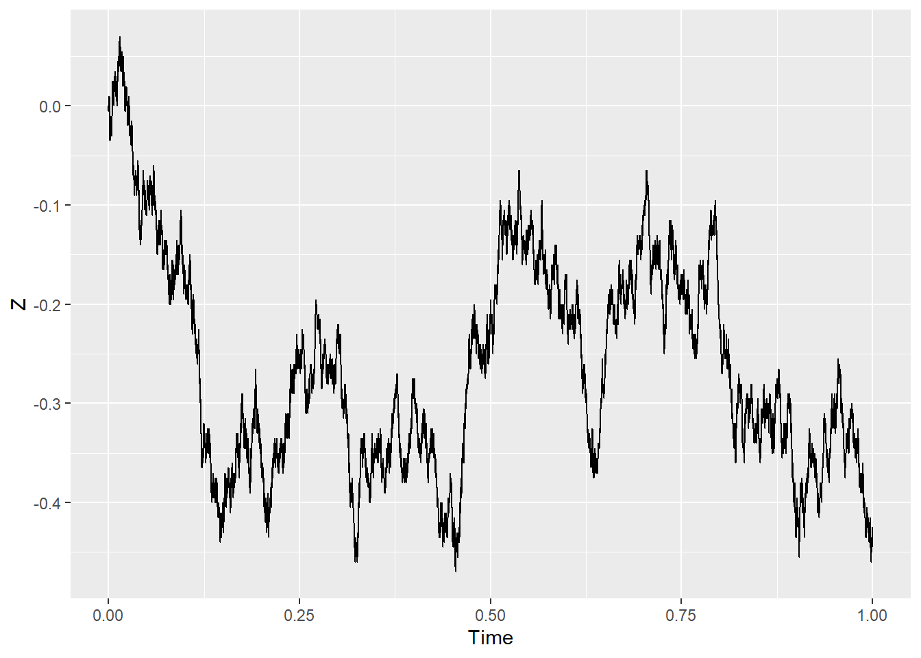
Let’s consider something else: let the random walk take more frequent and shorter steps. In the language of the symbols above, \(\Delta t\) and \(X_i\) are made smaller. As the steps become infinitesimals, the process becomes continuous. This is how a path may look like when \(\Delta t=0.1,\,0.01,\,0.001\):
A one-dimensional random walk from \(0\) to \(t\), in a similar fashion to the Central Limit Theorem, will converge to a normal variable:
\[
Z_t\sim \mathcal{N}(\mu=0,\sigma^2=t)
\]
These continuous-time stochastic processes are called Brownian motions or Wiener processes. They are denoted as \(B_t\) or \(W_t\) and fulfill a set of conditions:
\(B_0 = 0\)
Increments are independent, that is, \((B_{t+s} - B_t)\) doesn’t depend on earlier values \(B_r, \, r < t\)
Increments are Gaussian, that is, \((B_{t+s} - B_t) \sim \mathcal{N}(\mu=0,\sigma^2=s)\)
\(B_t\) is continuous at \(t\). A bit circular, I know.
There’s a catch, though. Even though they are continuous, these functions aren’t differentiable. You kind of see it from the previous path graphs, with how jagged they become as the indices, or steps, shrink. It also makes sense if you think about the way we constructed the process: when you are at a point in time \(t\), you don’t know from where you randomly came. Did you arrive from a smaller or bigger value at \(t-\Delta t\)? There’s no way to make sense of \(\frac{\partial Z_t}{\partial t}\).
Ito Calculus
The drunkard’s walk is a very simple case of a stochastic process. What about more complicated random variables or functions of these variables?
We start from a simple substitution: we can’t do \(\frac{\partial Z_t}{\partial t}\) but we “can” pass the \(dt\) as a multiplication, like we do with total derivatives, and refer to just \(dZ_t\). In general, we would like to express a minuscule change in the random variable being composed of something that changes very little in time and a little “noise”. In short, something like this:
\[
dZ_t = a(.)dt + b(.)dB_t
\]
For starters, we can assume the functions \(a\) and \(b\) above are only functions of time. We then integrate over time and reach the definition of an Ito process:
This representation is nice because the random variable \(Z_t\) has a mean that depends on something that changes along time, and has a variance tied to the noise. Having said that, we need a way to think about \(dB_t\) . For that, we can assume something simple, that instead of a continuum of \(dB_t\), there’s a list of discrete \(t_i\) and discrete increments \(\Delta B_{t_i}\), so now we deal with:
\[
\sigma_{t_{i}} * (B_{t_i}-B_{t_{i-1}})
\]
We can calculate the above because that difference of Brownian motions can be transformed into a normal distribution that we can manipulate. To show how this help us, we can do the following calculation and confirm that the expected value of \(Z\) only depends on the first term:
With these tools, we can calculate a mean and a variance for every point in time in a process. But there’s an even more powerful tool in our arsenal: Ito’s lemma, or Ito’s formula. In order to present this, we start with an Ito process for a random variable, say \(X_t\):
The first equation almost looks like a Taylor expansion up to the 2nd derivative, and in informal proofs that’s what’s going on. The second equation shows the explicit expressions for the \(a(t,X_t)\) and \(b(t,X_t)\) functions we mentioned before. This is great, because we can still split the “trend” component and the “noise” component for more complicated random processes. It also means that the “trend” is affected by how strong the “noise” is. Finally, notice that a non-random function with \(\sigma_t=0\) reverts to a classical total derivative and chain rule.
Martingales and final notions
Some stochastic processes present additional properties. One of those “some” are the martingales. They are either discrete or continuous-time processes that satisfy:
\(\mathbb{E}[|X_t|]<\infty, \forall t \ge 0\) . This means that the process always has a finite value.
\(\mathbb{E}[X_{t+s}|X_t]=X_t, \forall t \le s\). This means that the expected value for future realizations of the process is whatever value you have right now.
The drunkard’s walk is an example of a martingale: at any time, it’s equally likely it will go up or down, so the expected value is wherever you are at that point in time. Brownian motions are also martingales: increments follow a normal distribution, so the expected value of the increment is \(0\). Other examples of typical martingales are betting black or red at the roulette, or a stock price in the short term.
There’s a result called the Martingale Representation Theorem, which states that any random variable \(X\) can be written in terms of another process \(C\), with values known in advance, like so:
\[
X = \mathbb{E}\left[X\right] + \int_0^\infty C_s\,dB_s
\]
This is valuable for finance people because it means that any investment strategy (which is a random process) can be replicated with a different investment strategy (another process), but with lower volatility (and probably higher initial cost!). This theorem is less valuable because it doesn’t give any means to calculate it, we can’t apply a derivative and try to extract that \(dB_t\)
A second representation, from Rogers and Williams (2000), establishes that martingales can be represented as Ito integrals:
\[
M_t = M_0 + \int_0^t \alpha_s\,dB_s
\]
In a limited sense, \(\alpha_t\) can be thought as \(\frac{\partial M_t}{\partial t}\) because if we integrate it up to \(t\) we recover the final point, but it’s not quite what we are looking for.
And it’s always frustrating. We have been trying to find a way to calculate derivatives on these random processes, Brownian motions and martingales, but it’s elusive. And the thing is, we kind of know that is possible. Indeed, let’s go back to our first continuous random process, the one-dimensional Wiener process. We managed to reach the point were we can say that \(W_t\) had a normal distribution. So, nothing prevents us from taking a derivative over that, right?
And there we have it. Ugly as it may be, we have constructed a derivative for how the density of these random variables evolve with time, although we don’t know if it’s even useful. Let’s plot it both the density and the derivative in 3D.
At this point, we have seen enough. We know what we want: a way to calculate derivatives over random variables and Wiener processes “in a certain sense” that’s useful. That’s what Malliavin calculus is set to do.
Rogers, L. C. G., and David Williams. 2000. Diffusions, Markov Processes and Martingales. 2nd ed. Vol. 2. Cambridge Mathematical Library. Cambridge University Press. https://doi.org/10.1017/CBO9780511805141.