Up until now, Malliavin calculus has been mostly a game or procedure we apply to stochastic processes. We will dive deeper and reach some interesting results.
Malliavin derivative of the Ornstein-Uhlenbeck process
Let’s consider a random process \(N_t\) that fluctuates around a value \(\mu\) and corrects itself more strongly the farther it is to \(\mu\), plus some noise. So, we want something like this:
\[
dN_t = \theta(\mu - N_t)\,dt+ \sigma\,dW_t
\]
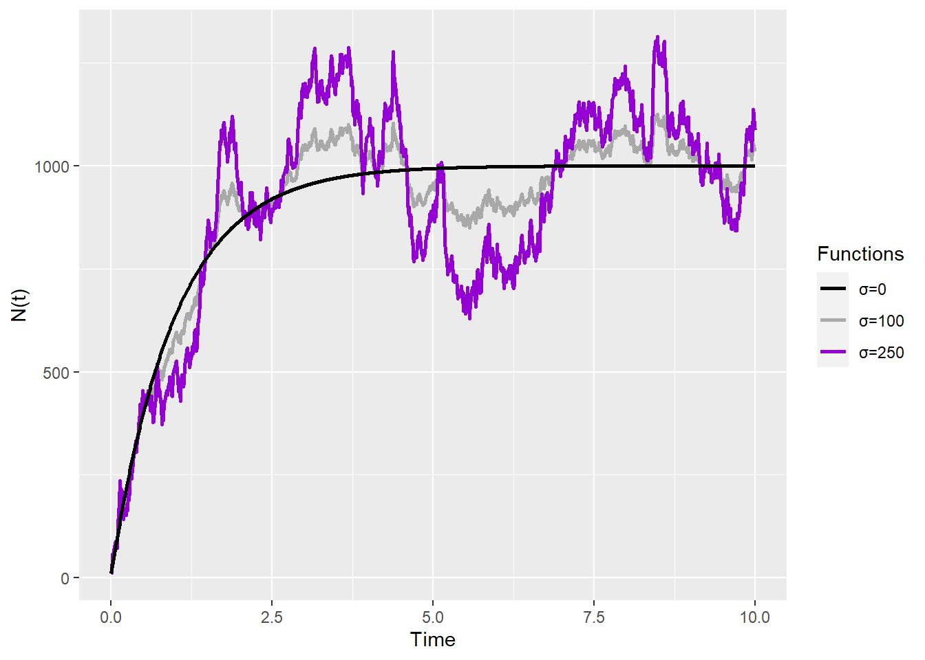
For example, let’s say that a lake can accept around \(\mu=1000\) trouts. If there are more than that, some will starve and die off, and if there are less, then they will reproduce. Finally, \(\theta\) controls how strong is the correction. Here are some examples with \(\theta=1\) and different values for \(\sigma\):
This is a very common process, so much it has a name: the Ornstein-Uhlenbeck process. Now, let’s calculate \(DN\). We have \(a(X) = \theta(\mu - X)\) and \(b(x) = \sigma\), so it’s not a simple Ito process that only depends on time. We better start from those before tackling the Ornstein-Uhlenbeck process. If we remember that we can split the integrals as \(\int_0^t... dW_t=\sum_{i=1}^n{...(W_{t_i}-W_{t_{i-1}})}\), then we can transform a classical Ito process \(X_t\) into something we can easily apply chain and product rules:
It looks messy, but things are what we expect: \(t\) is the terminal value of both integrals, \(s\) is the variable we use to integrate from \(0\) to \(t\), and \(r\) is the variable we introduced with the Malliavin Derivative. See that it makes sense: the influence of \(\sigma\) in the Ito process is the same along the whole Ito process path.
Now, we can use a similar argument for the number of trouts in the lake, which followed an Ornstein-Uhlenbeck process. Given that \(\mu_s\) and \(\sigma_s\) are now \(a(s,X_s)\) and \(b(s,X_s)\), we apply chain and product rules as above to arrive to:
In the case above, we arrive at a neat expression that tell us something interesting: the effect of a perturbation on the number of trouts is exponentially smaller if \(r<<t\). This makes sense: the population of trouts \(N\) wants to be close to \(\mu\) and the population from a distant past is irrelevant. It also tells us that there’s no randomness in the fluctuation because it doesn’t depend on any random variable, such as \(W_t\).
Finally, we lucked out above. The expression for \(D_rN_t\) is simple, so we could write an analytic expression for it. If it were more convoluted, it’s probably better to estimate a solution. Alos (2021) does a great job showcasing the above.
Clark-Ocone-Haussman Formula
Let’s see a relatively simple application with profound implications, following Friz (2002) entirely. Let’s consider this function:
Now, this is only valid at \(t=1\), but we use the expectation operator and martingale property to get the values at a previous time. We will call \(\mathcal{F}_s\) the filtration up to time \(s\), and it’s the way we call the “history” or “information” known up to time \(s\), and then:
Now, we pull everything together. This martingale \(F(t)\) is the solution of the (stochastic) differential equation \(dF(t) = h(t)F(t)dB_t\), when \(F(0)=1=\mathbb{E}[F]\). Replacing with the above expression we get:
This is the Clark-Ocone formula, which is an explicit formula for the Martingale Representation Theorem. The Malliavin derivative is the key ingredient to have an analytic expression and it’s the main reason one would care about it. What this is telling us is that any random variable indexed by time \(F_t\) can be split into a sum of a “deterministic” portion, the expected value, and a martingale that fluctuates around it.
We can apply this to the Ornstein-Uhlenbeck process for our trouts. We know from before that \(D_rN_t = \sigma\,e^{-\theta(t-r)}\). Notice that there’s no \(W_t\), so the expected value is just the Malliavin derivative. We could estimate the value of \(\mathbb{E}[N]\) or try to solve the (stochastic) differential equation, but given that the process already has a known solution, I’ll go ahead and add it. Here’s in all its splendor:
Why do we care about this? Well, for once, if we wanted to simulate different paths of our fish population \(N\), we only need to simulate the martingale portion, and the deterministic portion is only calculated once. Secondly, we can use the Clark-Ocone formula to directly calculate the variance for \(N\), without knowing the full analytic solution. Indeed, remember that \(\mathbb{Var}[N]=\mathbb{E}[N-\mathbb{E}[N]]^2\), so then, using Ito’s Isometry:
Notice that this works for any variable: you only need the Malliavin Derivative to get the variance. We see above that:
Our trout population \(N\) in the long term (\(t \rightarrow \infty\)) will be a process moving around \(\mu\) with a constant variance \(\frac{\sigma^2}{2\theta}\)
Variance at the time of trout introduction (\(t \approx 0\)) is very small because the growth of \(N\), trying to reach \(\mu\) as soon as possible, dominates over the noise
A large \(\theta\) will not only make the long term variance arrive sooner, it will also prevent large deviations from \(\mu\)
Alos, & Lorite, E. 2021. Malliavin Calculus in Finance: Theory and Practice (1st Ed.). 1st ed. Financial Mathematics Series. Chapman; Hall/CRC. https://doi.org/10.1201/9781003018681.